SUMIFS Function


The Excel SUMIFS function is similar to the SUMIF function
It adds up the values from a given range that meets multiple criteria.
The syntax for the SUMIFS function is:

=SUMIFS(sum_range, criteria_range1, criteria1, ...)

A)Sum_range =  The range of cells containing the values you want to add
B) Criteria_range = The range of cells containing the records you want to check against the criteria
C) Criteria = The criteria to determine whether the value is added or not

The example below shows the SUMIFS function being used to sum the order amounts by the company Carpet World.


Excel FLOOR Functions


In Excel we can use the FLOOR function to calculate this value.


 For example:


Say our price is Rs 4.32 and we need to round it down to the nearest value divisible by 5 cents, 
The FLOOR function would read:


=FLOOR(4.32, 0.05)
=Rs 4.30


Excel CEILING Function


Excel provides list of mathematical functions which enables you to evaluate complex logic instantly. From the list of functions provided, finding out Ceiling value would be useful, especially when you need to find it out for specified “multiple”. Excel 2010 CEILING function immediately evaluate the ceiling value based on specified multiple.

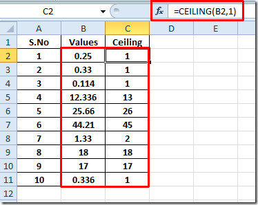
Launch Excel spreadsheet on which you want to apply ceiling function. For instance we have included a spreadsheet containing fields;


S.No, Values, and Ceiling.


Now we want to find out the ceiling of the data present in Values field. For this we will be using ceiling function, The syntax of the function is;
=CEILING(number,significance)

The first argument is number which refers to number for which you want to show ceiling of, and significance refers to any number of which nearest multiple is needed.

We will be writing this function as;

=CEILING(A1,2)

The first argument is A1 which refers to location of the cell, however you can put in values directly. The second argument is 2 which refers to nearest multiple of 2. 

As shown below, it yields 16 for the data 15 in Values field. It searched for the nearest significant value which is multiple to 15, the options would be 14 and 16 nearest to value 15, as we are finding out ceiling that’s why it shows 16 as a result.


Now for applying it over the field just drag down the plus sign at the end of the cell towards the end of the column


Now if you want to show the nearest whole number ceiling value, then just change the significance in the function to 1. It would be useful for decimal values.


For finding out ceiling of the value exclusively you need to put in first argument directly.


Sum or Count cells that have a specified Fill Color


CUSTOM COLOR FUNCTION:

This can be done with the aid of a Custom Function.  A custom function, also called a User Defined Function, is a function that we write ourselves using VBA

There is no built-in excel function to do this. But you can use a UDF that
looks at the range and returns the sum of color. But that function will not
recalculate if you change color. Every time you change the color you will
need to recalculate or wait excel to recalculate...


It is possible to calculate data based on cell color in excel by

SUM

=ColorFunction(I12,G7:G12,TRUE)

COUNT

=ColorFunction(I12,G7:G12,FALSE)


<!===========Excel macro code start===========>

The Code:
Function SumColor(rColor As Range, rSumRange As Range)

''''''''''''''''''''''''''''''''''''''
'Written by Senthamaraikannan
'www.askannan.blogspot.com

'Sums cells based on a specified fill color.
'''''''''''''''''''''''''''''''''''''''
 Dim rCell As Range
 Dim iCol As Integer
 Dim vResult

 iCol = rColor.Interior.ColorIndex

  For Each rCell In rSumRange
   If rCell.Interior.ColorIndex = iCol Then
    vResult = WorksheetFunction.Sum(rCell) + vResult
   End If
  Next rCell

 SumColor = vResult
End Function

<!=========Excel macro code End===============>

Download Excel Example file here

Convert Numbers to Words


With the custom functions, SpellNumber, GetHundreds, GetTens, and GetDigit, you can convert a numeric value into its equivalent in English words.
For example, you can change 35.50 into the following text: Thirty Two Dollars and Fifty Cents, by entering the following formula into a cell:
=SpellNumber(35.50)
You can also use these functions to refer to other cells in the workbook. For example if the number 35.50 was in A1, you could type the following into a cell:
=SpellNumber(A1)
I have requests to convert this to other languages; sorry my language skills are lacking. I also do not know how nor can fathom negative numbers.
Example:
CODE:-
<!====================Macro code start here=============>
Option Explicit

'****************
' Main Function *
'****************
Function SpellNumber(ByVal MyNumber)
    Dim Dollars, Cents, Temp
    Dim DecimalPlace, Count

    ReDim Place(9) As String
    Place(2) = " Thousand "
    Place(3) = " Million "
    Place(4) = " Billion "
    Place(5) = " Trillion "

    ' String representation of amount
    MyNumber = Trim(Str(MyNumber))

    ' Position of decimal place 0 if none
    DecimalPlace = InStr(MyNumber, ".")
    'Convert cents and set MyNumber to dollar amount
    If DecimalPlace > 0 Then
        Cents = GetTens(Left(Mid(MyNumber, DecimalPlace + 1) & "00", 2))
        MyNumber = Trim(Left(MyNumber, DecimalPlace - 1))
    End If

    Count = 1
    Do While MyNumber <> ""
       Temp = GetHundreds(Right(MyNumber, 3))
       If Temp <> "" Then Dollars = Temp & Place(Count) & Dollars
          If Len(MyNumber) > 3 Then
             MyNumber = Left(MyNumber, Len(MyNumber) - 3)
        Else
            MyNumber = ""
        End If
        Count = Count + 1
    Loop

    Select Case Dollars
        Case ""
            Dollars = "No Dollars"
        Case "One"
            Dollars = "One Dollar"
        Case Else
            Dollars = Dollars & " Dollars"
    End Select

    Select Case Cents
        Case ""
            Cents = " and No Cents"
        Case "One"
            Cents = " and One Cent"
        Case Else
            Cents = " and " & Cents & " Cents"
    End Select

    SpellNumber = Dollars & Cents
End Function

'*******************************************
' Converts a number from 100-999 into text *
'*******************************************
Function GetHundreds(ByVal MyNumber)
    Dim Result As String

    If Val(MyNumber) = 0 Then Exit Function
    MyNumber = Right("000" & MyNumber, 3)

    'Convert the hundreds place
    If Mid(MyNumber, 1, 1) <> "0" Then
        Result = GetDigit(Mid(MyNumber, 1, 1)) & " Hundred "
    End If

    'Convert the tens and ones place
    If Mid(MyNumber, 2, 1) <> "0" Then
        Result = Result & GetTens(Mid(MyNumber, 2))
    Else
        Result = Result & GetDigit(Mid(MyNumber, 3))
    End If

    GetHundreds = Result
End Function

'*********************************************
' Converts a number from 10 to 99 into text. *
'*********************************************
Function GetTens(TensText)
    Dim Result As String

    Result = ""           'null out the temporary function value
    If Val(Left(TensText, 1)) = 1 Then   ' If value between 10-19
        Select Case Val(TensText)
            Case 10: Result = "Ten"
            Case 11: Result = "Eleven"
            Case 12: Result = "Twelve"
            Case 13: Result = "Thirteen"
            Case 14: Result = "Fourteen"
            Case 15: Result = "Fifteen"
            Case 16: Result = "Sixteen"
            Case 17: Result = "Seventeen"
            Case 18: Result = "Eighteen"
            Case 19: Result = "Nineteen"
            Case Else
        End Select
      Else                                 ' If value between 20-99
        Select Case Val(Left(TensText, 1))
            Case 2: Result = "Twenty "
            Case 3: Result = "Thirty "
            Case 4: Result = "Forty "
            Case 5: Result = "Fifty "
            Case 6: Result = "Sixty "
            Case 7: Result = "Seventy "
            Case 8: Result = "Eighty "
            Case 9: Result = "Ninety "
            Case Else
        End Select
         Result = Result & GetDigit _
            (Right(TensText, 1))  'Retrieve ones place
      End If
      GetTens = Result
   End Function

'*******************************************
' Converts a number from 1 to 9 into text. *
'*******************************************
Function GetDigit(Digit)
    Select Case Val(Digit)
        Case 1: GetDigit = "One"
        Case 2: GetDigit = "Two"
        Case 3: GetDigit = "Three"
        Case 4: GetDigit = "Four"
        Case 5: GetDigit = "Five"
        Case 6: GetDigit = "Six"
        Case 7: GetDigit = "Seven"
        Case 8: GetDigit = "Eight"
        Case 9: GetDigit = "Nine"
        Case Else: GetDigit = ""
    End Select
End Function
<!=========Macro code end here===============>

Download Example excel file

Custom Cell Formatting


Custom Cell Formatting
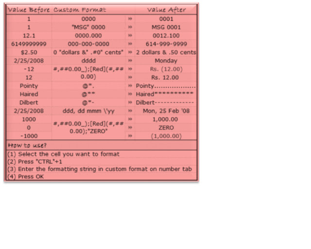
First take a look at how the cell formatting dialog box – number tab looks like:


Now apart from the built in types General (leave excel to guess the data format), number, currency, accounting (uses the separators, () notation etc.), date, time, percentage, fraction, scientific, text there are 2 interesting types of formating.

Custom: Used for creating your own cell formatting structure. This is a bit like regular expressions but in entire microsoftish way.
Any cell custom format code will be divided in to 4 parts : positive numbers ; negative numbers ; zeros ; text. If your formatting codes have less number of parts (say 1 or 2 or 3) excel will use some common sense to find out which ones are for what.
This is probably how you can use the custom cell formatting feature in Microsoft excel.


Excel Rounding to nearest multiple of XX


Excel Rounding to nearest multiple of XX 

Given a column of numbers
 we want to round to the nearest multiple of 5 Or 50

EXAMPLE :
If you have the analyst tool pak installed, use
=MROUND(A1,5)
=MROUND(A1,50)
Otherwise you could use
=ROUND(A1/5,0)*5
=ROUND(A1/50,50)*50

Round a number to a specified multiple


Round a number to a specified multiple
To do this task, use the MROUND function.
EXAMPLE
The example may be easier to understand if you copy it to a blank worksheet.

1
2
3
4
5
A
B
Formula
Description (Result)
=MROUND(16, 5)
Rounds 16 to a nearest multiple of 5 (15)
=MROUND(-16, -5)
Rounds -16 to a nearest multiple of -5 (-15)
=MROUND(2.6, 0.08)
Rounds 2.6 to a nearest multiple of 0.08 (2.64)
=MROUND(5, -2)
Returns an error, because 5 and -2 have different signs (#NUM!)

Round a number to a significant digit above 0


Round a number to a significant digit above 0
To do this task, use the ROUND, ROUNDUP, ROUNDDOWN, LEN, and INT functions.
EXAMPLE
The example may be easier to understand if you copy it to a blank worksheet.

1
2
3
A
Data
5492820
22230
Formula
Description (Result)
=ROUND(A2,3-LEN(INT(A2)))
Rounds the top number to 3 significant digits (5490000)
=ROUNDDOWN(A3,3-LEN(INT(A3)))
Rounds the bottom number down to 3 significant digits (22200)
=ROUNDUP(A2,5-LEN(INT(A2)))
Rounds the top number up to 5 significant digits (5492900)

Round a number to the nearest number


Round a number to the nearest number
To do this task, use the ROUND function.
EXAMPLE
The example may be easier to understand if you copy it to a blank worksheet.

1
2
3
4
A
Data
20.3
5.9
-5.9
Formula
Description (Result)
=ROUND(A2,0)
Rounds 20.3 down, because the fractional part is less than .5 (20)
=ROUND(A3,0)
Rounds 5.9 up, because the fractional part is greater than .5 (6)
=ROUND(A4,0)
Rounds -5.9 down, because the fractional part is less than -.5 (-6)

Round a number to a near fraction


Round a number to a near fraction
To do this task, use the ROUND function.
EXAMPLE
The example may be easier to understand if you copy it to a blank worksheet.

1
2
3
A
Data
1.25
30.452
Formula
Description (Result)
=ROUND(A2,1)
Rounds the number to the nearest tenth (one decimal place). Because the portion to be rounded is 0.05 or greater, the number is rounded up (result: 1.3)
=ROUND(A3,2)
Rounds the number to the nearest hundredth (two decimal places). Because the portion to be rounded, 0.002, is less than 0.005, the number is rounded down (result: 30.45)

Round a number down


Round a number down
To do this task, use the ROUNDDOWN function.
EXAMPLE
The example may be easier to understand if you copy it to a blank worksheet.

1
2
3
4
A
Data
20.3
-5.9
12.5493
Formula
Description (Result)
=ROUNDDOWN(A2,0)
Rounds 20.3 down to the nearest whole number ( 20)
=ROUNDDOWN(A3,0)
Rounds -5.9 down (-5)
=ROUNDDOWN(A4,2)
Rounds the number down to the nearest hundredth, two decimal places ( 12.54)


Round a number up


Round a number up
To do this task, use the ROUNDUP, EVEN, or ODD functions.
EXAMPLE
The example may be easier to understand if you copy it to a blank worksheet.

1
2
3
4
A
Data
20.3
-5.9
12.5493
Formula
Description (Result)
=ROUNDUP(A2,0)
Rounds 20.3 up to the nearest whole number (21)
=ROUNDUP(A3,0)
Rounds -5.9 up (-6)
=ROUNDUP(A4,2)
Rounds 12.5493 up to the nearest hundredth, two decimal places (12.55)
=EVEN(A2)
Rounds 20.3 up to the nearest even number (22)
=ODD(A2)
Rounds 20.3 up to the nearest odd number (21)


About Me

My photo
I`m Author of Senthamaraikannanclub and i loves blogging and Socila networking .,
counter

VISITORS