Excel CEILING Function

Excel provides list of mathematical functions which enables you to evaluate complex logic instantly. From the list of functions provided, finding out Ceiling value would be useful, especially when you need to find it out for specified “multiple”. Excel 2010 CEILING function immediately evaluate the ceiling value based on specified multiple.

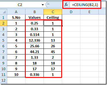
Launch Excel spreadsheet on which you want to apply ceiling function. For instance we have included a spreadsheet containing fields;

S.No, Values, and Ceiling.

Now we want to find out the ceiling of the data present in Values field. For this we will be using ceiling function, The syntax of the function is;

=CEILING(number,significance)

The first argument is number which refers to number for which you want to show ceiling of, and significance refers to any number of which nearest multiple is needed.

We will be writing this function as;

=CEILING(A1,2)

The first argument is A1 which refers to location of the cell, however you can put in values directly. The second argument is 2 which refers to nearest multiple of 2. 

As shown below, it yields 16 for the data 15 in Values field. It searched for the nearest significant value which is multiple to 15, the options would be 14 and 16 nearest to value 15, as we are finding out ceiling that’s why it shows 16 as a result.

Now for applying it over the field just drag down the plus sign at the end of the cell towards the end of the column

Now if you want to show the nearest whole number ceiling value, then just change the significance in the function to 1. It would be useful for decimal values.

For finding out ceiling of the value exclusively you need to put in first argument directly.

Categories: FORMULA